 duydl
duydl 

This year marks the 20th anniversary of Google Summer of Code (GSoC), with 195 open-source organizations developing various impactful projects. As part of 1,200 contributors, I had the opportunity to work with Machine Learning for Science (ML4Sci), an organization that applies state-of-the-art machine learning techniques to solve cutting-edge problems in science. My project, titled "Quantum Contrastive Representation Learning for High-Energy Physics (HEP)," involved developing machine learning models—both classical and quantum—to learn useful representations from data for various downstream tasks such as classification, regression, and generation.
Project Objectives
The focus of this project was to investigate various architectures and pipelines for contrastive learning, as well as the opprotunities and effect of integrating quantum computing methods. The primary pipelines I explored included:
-
Supervised Contrastive Learning: In this method, we attempt to learn useful representations by using a metric instead of, for example, directly predicting a likelihood. The pretrained model is then used to generate embeddings as inputs to simple linear probing methods for downstream tasks.
-
Self-Supervised Contrastive Learning: In this method, we attempt to learn useful representations without labels, where similar and dissimilar pairs are generated using augmentations. The learned representations can then be fine-tuned with labels for downstream tasks like classification.
For both pipelines, I explored different types of architectures including Convolutional Neural Networks (CNNs) and Graph Neural Networks (GNNs). Additionally, I incorporated Quantum Variational Circuits into some of these models to see whether quantum computing could offer an advantage. My work also extended to exploring model-based augmentations for graph data, namely rationale discovery, which is shown to be particularly advantageous with graph distributions that is not understood well enough for effective augmentations.
Datasets
A significant aspect of the project was working with diverse datasets, each posing its own challenges:
-
Simple Image Classification: I used datasets like MNIST and Fashion MNIST to benchmark initial models, given their simplicity and widespread use in machine learning research.
-
High-Energy Physics (HEP) Datasets: These included images from the LHC experiments, specifically the Track, ECAL, and HCAL components, as well as synthetic particle jets generated by PYTHIA. The Photo-Electron and Quark-Gluon datasets were used for classification tasks, as they represent different particle interactions in the detector.
-
Quantum Machine Molecular Energy (QM7): For regression tasks, I experimented with the QM7 dataset, which consists of molecules with associated formation energies. This dataset provided an excellent benchmark for testing how well models can learn from small-scale quantum mechanical data.
1. Simple Image Classification Datasets: MNIST & Fashion MNIST
To establish a baseline for model performance, I began with simpler, widely-used datasets such as MNIST and Fashion MNIST. These datasets are often used to benchmark image classification models and contrastive learning frameworks due to their accessibility and straightforward structure.
- MNIST contains 70,000 grayscale images of handwritten digits, each 28x28 pixels, and is used extensively in machine learning research as a starting point for validating models.
- Fashion MNIST, a similar dataset, consists of 70,000 grayscale images of clothing items. It introduces a slightly higher level of complexity than MNIST, as it involves classifying 10 categories of fashion items rather than digits.
These datasets were ideal for experimenting with basic Convolutional Neural Networks (CNNs) and testing out early versions of contrastive learning models.
2. High-Energy Physics (HEP) Datasets
A key focus of this project was analyzing complex datasets from high-energy physics (HEP) experiments, particularly from the Large Hadron Collider (LHC) at CERN. The LHC is a massive particle accelerator that collides particles at nearly the speed of light to explore fundamental questions about the universe, such as understanding the building blocks of matter and the forces that govern them. By accelerating particles in a 27-kilometer ring, it allows scientists to study the results of these high-energy collisions, which have led to important discoveries like the Higgs boson.
One of the main experiments at the LHC is the CMS (Compact Muon Solenoid) detector. This detector is a large, layered structure designed to track and analyze particles produced in collisions. As particles fly out from the collision point, their trajectories and energies are measured with extreme precision using components such as: - Tracker: Identifies the path of charged particles. - Electromagnetic Calorimeter (ECAL): Measures the energy of particles like electrons and photons. - Hadron Calorimeter (HCAL): Detects composite particles, such as quarks and gluons, which interact through the strong force.
These components work together to capture detailed data from the collisions, allowing researchers to study the behavior of particles. The challenge is to process this data efficiently and use machine learning to distinguish between different types of particle events.
Quark-Gluon Dataset from CMS
The Quark-Gluon Dataset is a simulated dataset derived from the data collected by the CMS detector. It consists of over 933,000 images, each 125x125 pixels in size, with three channels that correspond to measurements from the Tracker, ECAL, and HCAL components. Each image represents a snapshot of the energy distribution in a particle collision, and the goal is to classify whether the collision produced a quark-initiated jet or a gluon-initiated jet.
- Quarks: Fundamental particles that form protons and neutrons, which make up the atomic nucleus. Quarks are the "building blocks" of matter.
- Gluons: Force-carrying particles that mediate the strong force between quarks. They act as the "glue" that holds quarks together inside protons and neutrons.
Understanding the difference between quark and gluon jets is crucial in particle physics because quarks and gluons behave differently when they are produced in high-energy collisions. Quark-initiated jets tend to produce fewer, more energetic particles, while gluon-initiated jets produce more particles with lower energy. Being able to distinguish between the two is important for understanding the processes happening inside the detector and for analyzing the results of particle collisions more accurately.
This dataset presents a significant challenge due to the complexity and high-dimensional nature of the data. Unlike simpler image datasets like MNIST, where the patterns are more easily recognized, the Quark-Gluon Dataset requires more sophisticated models to capture the underlying structure of the particle collisions. Models like Graph Neural Networks (GNNs), which can model relationships between particles, and Hybrid Quantum Models, which explore the potential advantages of quantum computing, were used to tackle these challenges. While traditional models like Convolutional Neural Networks (CNNs) performed well on simpler datasets, they struggled with the complexities of the Quark-Gluon data, highlighting the need for more advanced approaches.
HEP PYTHIA Synthetic Particle Jets
In addition to real experimental data, synthetic particle jets were generated using the PYTHIA event generator, a widely used tool for simulating particle collisions in high-energy physics. These particle jets consist of multiple physical properties for each particle in the jet, represented as 4-tuples: transverse momentum (pT), rapidity (y), azimuthal angle (ϕ), and particle ID.
The task was to classify whether each jet was quark- or gluon-initiated, and this dataset further validated the model’s ability to process particle-level data using GNNs and hybrid quantum models. A preprocessed version of the original dataset is also available with 12,500 jets, each converted into graph-based data with 8 features per node, capturing the following derived properties:
- \(p_T\): Transverse Momentum — Measures how much momentum a particle has perpendicular to the collision axis (beamline). This helps in understanding the energy distribution in the transverse plane.
- \(y\): Rapidity — Describes how the particle’s velocity compares to the speed of light along the direction of motion, offering insights into the particle’s energy and momentum.
- \(\phi\): Azimuthal Angle — The angle in the transverse plane, ranging from 0 to \(2\pi\), indicating the particle's direction relative to the beamline.
- \(m\): Rest Mass — The intrinsic mass of the particle when it is at rest.
- \(E\): Total Energy — The sum of the particle’s kinetic and potential energy.
- \(p_x\): Momentum along the x-axis — The x-component of the particle’s momentum vector.
- \(p_y\): Momentum along the y-axis — The y-component of the particle’s momentum vector.
- \(p_z\): Momentum along the z-axis — The z-component of the particle’s momentum vector.
Each jet is represented as a graph where the nodes correspond to particles, and the edges represent the relationships between them. The task was to classify these jets into two classes: quark-initiated or gluon-initiated. Quark jets tend to have fewer, more energetic particles, while gluon jets have more particles with lower energy.
3. Quantum Machine Molecular Energy (QM7) Dataset
For regression tasks, I turned to the Quantum Machine 7 (QM7) dataset. This dataset consists of 7,165 molecules, each represented by its atomic coordinates and corresponding formation energy—a crucial property in quantum chemistry that reflects the stability of a molecule.
- Formation energy is the energy required to form a compound from its constituent atoms, and predicting this accurately is critical in areas like materials discovery and drug design.
The challenge was to predict the formation energy for these molecules using contrastive learning methods. The QM7 dataset is relatively small, but it provided a perfect testing ground for the quantum variational circuits integrated into the machine learning models. By combining Graph Neural Networks (GNNs) with quantum models, I aimed to improve the model's performance in predicting molecular properties.
While the Mean Absolute Error (MAE) results from the quantum models were comparable to classical methods, further optimization is required to fully explore the potential of quantum models in this domain.
Contrastive Losses
Implementations
Contrastive losses are the core mechanism for our approach of representation learning. The implementation often involves several key components that work together to optimize the embedding space and improve the learning process, such as distances, miners, and reducers.
The distance function is a crucial part of the contrastive loss. It measures the similarity or dissimilarity between embeddings in the latent space. Common choices include: - Euclidean distance: Measures the straight-line distance between two embeddings. It's often used for calculating how "far apart" two points are in the latent space. - Cosine similarity: Computes the cosine of the angle between two embeddings. This is especially useful when the direction of the embeddings is more important than their magnitude.
Miners is the optional component but they can significantly improve the efficiency and effectiveness of the training process by identifying the most informative pairs for training. In a batch of data, not all positive or negative pairs contribute equally to the learning process. Some pairs are already well separated or clustered, so focusing on them may not improve the model much.
Reducers control how the loss is calculated and aggregated across the batch. They could, additionally, apply techniques like regularization, which limits the impact of outliers so no single pair dominates the loss function, or weighted loss, which assigns different importance to pairs, ensuring that the most informative or challenging examples are prioritized during training.
In a typical contrastive learning workflow: 1. Embeddings are generated by the model, with a shape of \((N, \text{embedding\_size})\), where \(N\) is the batch size. 2. Distances are computed between positive and negative pairs in the embedding space. 3. Miners identify the most challenging pairs within the batch (hard positives and hard negatives). 4. Reducers aggregate the loss across the batch, ensuring that hard examples are emphasized, and regularization is applied.
Through iterative updates, the model learns to create a more discriminative and robust feature space, fascilitating downstream tasks like classification or clustering.
Examples
While there are several types of contrastive losses, we focused on a few key variants, revisiting the writing from midterm report.
Pair Contrastive Loss
Pair contrastive loss is designed to minimize the distance between positive pairs and separate negative pairs by a specified margin \(m\). The general form of the loss is:
Where: - \(y_{ij}\) is a binary label (1 for positive pairs, 0 for negative pairs). - \(d(x_i, x_j)\) is the distance between embeddings (e.g., Euclidean or cosine). - \(m\) is the margin that controls how far apart negative pairs should be.
Alternative distance metrics, like cosine similarity, can also be used depending on the task, each with different advantages.
Temperature-Scaled Losses
Temperature-scaled losses, such as NT-Xent and InfoNCE, introduce a temperature parameter \(\tau\) to smooth the similarity distribution and emphasize harder negative examples. The InfoNCE loss is given by:
Where: - \(\text{sim}(z_i, z_j)\) is the cosine similarity between embeddings. - \(\tau\) controls the sharpness of the similarity distribution, making the model more sensitive to challenging examples.
Alignment and Uniformity
The alignment and uniformity metrics provide useful ways to evaluate how well the embedding space is structured: - Alignment loss ensures that positive pairs are closely clustered:
This metric minimizes the distance between positive pairs, improving representation quality.
- Uniformity loss measures how well the representations are distributed across the latent space:
It encourages embeddings to spread out across the space, maximizing utilization of the latent space.
The two losses can be combined:
This helps create a balanced embedding space where positive pairs are tightly clustered while maintaining good separation among negative pairs.
Quantum Fidelity
In quantum computing, fidelity measures the similarity between two pure quantum states. There are two primary ways to compute this: through direct fidelity calculation or using the SWAP test.
For two pure quantum states, (|\psi_1\rangle) and (|\psi_2\rangle), the fidelity is given by the squared magnitude of their inner product:
As full quantum states are usually not accessible, an approximation of fidelity can be computed using the Bhattacharyya coefficient:
Here, ( p_{1i} ) and ( p_{2i} ) are the probabilities of specific measurement outcomes for the two states.
On the other hand, the SWAP test is a quantum algorithm that estimates fidelity by using an ancillary qubit and performing controlled-SWAP operations between corresponding qubits of the two states. The fidelity is inferred from the probability of measuring the ancillary qubit in the ( |0\rangle ) state:
From this, the fidelity is:
In Pennylane, these approaches can be simulated to verify the theory:
-
Direct Fidelity Calculation: We can use
qml.state()to access the full quantum states and compute their inner product directly, orqml.probs()to extract the probability distributions and approximate fidelity using the Bhattacharyya coefficient. -
SWAP Test: The SWAP test can be implemented with controlled-SWAP gates and an ancillary qubit to estimate fidelity based on the measurement probability of the ancillary qubit.
Here, these methods are implemented and tested in Pennylane:
import pennylane as qml
from pennylane import numpy as np

# Define quantum devices
dev1 = qml.device('default.qubit', wires=3)
dev2 = qml.device('default.qubit', wires=3)

# Define two circuits
@qml.qnode(dev1)
def circuit1():
    qml.Hadamard(wires=0)
    qml.CNOT(wires=[0, 1])
    qml.CNOT(wires=[1, 2])
    qml.Hadamard(wires=2)
    return qml.probs(wires=[0, 1, 2])

@qml.qnode(dev2)
def circuit2():
    qml.PauliX(wires=0)
    qml.CNOT(wires=[0, 1])
    qml.CNOT(wires=[1, 2])
    qml.Hadamard(wires=2)
    return qml.probs(wires=[0, 1, 2])
    # return qml.state()

# qml.density_matrix(wires=[0, 1, 2])
# qml.sample(qml.PauliZ(0))
# qml.expval(qml.PauliZ(0))

# Get the quantum states from each circuit
state1 = circuit1()
state2 = circuit2()

print("State 1 and State 2:")
print(state1, state2)
# Compute the direct fidelity between the two states
fidelity_direct = np.sum(np.sqrt(state1 * state2)) ** 2 # qml.probs
# fidelity_direct = np.abs(np.dot(np.conj(state1), state2)) ** 2 # qml.state()

print(f"Direct Fidelity: {fidelity_direct}")
# Define a SWAP test circuit with 7 qubits (3 for each state + 1 ancillary)
dev_swap = qml.device('default.qubit', wires=7)

@qml.qnode(dev_swap)
def swap_test_circuit():
    # Apply Hadamard on the ancillary qubit
    qml.Hadamard(wires=0)

    # Prepare the first quantum state (on qubits 1, 2, 3)
    qml.Hadamard(wires=1)
    qml.CNOT(wires=[1, 2])
    qml.CNOT(wires=[2, 3])
    qml.Hadamard(wires=3)

    # Prepare the second quantum state (on qubits 4, 5, 6)
    qml.PauliX(wires=4)
    qml.CNOT(wires=[4, 5])
    qml.CNOT(wires=[5, 6])
    qml.Hadamard(wires=6)

    # Apply controlled SWAP gates between corresponding qubits
    qml.CSWAP(wires=[0, 1, 4])
    qml.CSWAP(wires=[0, 2, 5])
    qml.CSWAP(wires=[0, 3, 6])

    # Apply final Hadamard gate on the ancillary qubit
    qml.Hadamard(wires=0)

    # Measure the ancillary qubit
    return qml.probs(wires=0)

# Execute the SWAP test
probs = swap_test_circuit()

# Estimate fidelity using the SWAP test result
fidelity_swap = 2 * probs[0] - 1
print(f"Fidelity (SWAP Test): {fidelity_swap}")
The output is as follow when using qml.probs:
Circuit 1:
0: ──H─╭●───────┤ ╭Probs
1: ────╰X─╭●────┤ ├Probs
2: ───────╰X──H─┤ ╰Probs

Circuit 2:
0: ──X─╭●───────┤ ╭Probs
1: ────╰X─╭●────┤ ├Probs
2: ───────╰X──H─┤ ╰Probs
State 1 and State 2:
[0.25 0.25 0.   0.   0.   0.   0.25 0.25] [0.  0.  0.  0.  0.  0.  0.5 0.5]

SWAP Test Circuit:
0: ──H──────────╭●────╭●────╭●─────H─┤  Probs
1: ──H─╭●───────├SWAP─│─────│────────┤
2: ────╰X─╭●────│─────├SWAP─│────────┤
3: ───────╰X──H─│─────│─────├SWAP────┤
4: ──X─╭●───────╰SWAP─│─────│────────┤
5: ────╰X─╭●──────────╰SWAP─│────────┤
6: ───────╰X──H─────────────╰SWAP────┤
Fidelity (Direct Calculation): 0.4999999999999996
Fidelity (SWAP Test Estimation): 0.4999999999999989
and qml.state:
Circuit 1:
0: ──H─╭●───────┤  State
1: ────╰X─╭●────┤  State
2: ───────╰X──H─┤  State

Circuit 2:
0: ──X─╭●───────┤  State
1: ────╰X─╭●────┤  State
2: ───────╰X──H─┤  State
State 1 and State 2:
[ 0.5+0.j  0.5+0.j  0. +0.j  0. +0.j  0. +0.j  0. +0.j  0.5+0.j -0.5+0.j] [ 0.        +0.j  0.        +0.j  0.        +0.j  0.        +0.j
  0.        +0.j  0.        +0.j  0.70710678+0.j -0.70710678+0.j]

SWAP Test Circuit:
0: ──H──────────╭●────╭●────╭●─────H─┤  Probs
1: ──H─╭●───────├SWAP─│─────│────────┤
2: ────╰X─╭●────│─────├SWAP─│────────┤
3: ───────╰X──H─│─────│─────├SWAP────┤
4: ──X─╭●───────╰SWAP─│─────│────────┤
5: ────╰X─╭●──────────╰SWAP─│────────┤
6: ───────╰X──H─────────────╰SWAP────┤
Fidelity (Direct Calculation): 0.4999999999999998
Fidelity (SWAP Test Estimation): 0.4999999999999989
Architecture
1. Supervised and Unsupervised Contrastive Learning
During this phase, I further investigated the loss functions used in both supervised and unsupervised contrastive learning (CL). This exploration extended to both full quantum and hybrid models. The key focus was to evaluate how well different loss functions, such as temperature-scaled losses like InfoNCE and pairwise contrastive losses, could perform when integrated into hybrid classical-quantum networks. In particular, I analyzed how these loss functions influence the representations learned by classical models versus those augmented by quantum circuits.

2. Graph Processing for Quark-Gluon Jet Images
For the Quark-Gluon Jet (QJ) images, I moved beyond convolutional approaches and began exploring graph-based models to better capture the underlying structure of the data.

3. Quantum Integration
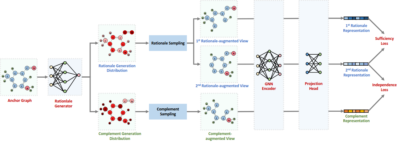
4. Rationale Discovery for Graph Contrastive Learning
In the final approach, I focused on model-based augmentations for unsupervised contrastive representation learning, particularly in tasks such as Quark-Gluon Jet classification and the Quantum Machine 7 (QM7) regression for predicting molecular formation energy. By generating synthetic data, I utilized model-based augmentation to better exploit unsupervised settings where direct label supervision is absent.
-
Rationale Generator: A model component assigns probability scores to each node, estimating its importance for the task. This helps determine which nodes will be retained for creating augmented views.
-
Positive Sample Generation (Rationale View): Based on the rationale generator’s output, high-probability nodes are retained, creating the rationale view, a smaller graph that still preserves the core, important information about the instance.
-
Negative Sample Generation (Complement View): Low-probability nodes or the complement of the rationale (the set of nodes that were discarded) are used to form a negative sample, called the complement view. This forces the model to contrast and learn the important features of the graph.
-
Graph Encoder: After generating the rationale and complement views, these two graphs are processed through the same encoder, producing two views (two sets of node embeddings). The encoder learns representations that emphasize important features in the rationale view while downplaying irrelevant ones in the complement view.
-
Contrastive Learning: The embeddings from the two views are passed to a combined loss function, to optimize the generator rationale of graph i.e importance of a node to represent an instance.
-
Sufficiency Loss: Ensures that the rationale (positive sample) contains enough information for the instance-discrimination task. It minimizes the negative log-likelihood of the correct prediction based on the rationale view:
$$ \mathcal{L}_{\text{sufficiency}} = - \log p(y \mid G_{\text{rationale}}) $$ -
Independence Loss: Ensures that the complement view (negative sample) does not contain sufficient information to predict the label. It maximizes the log-likelihood of the incorrect prediction for the complement view:
$$ \mathcal{L}_{\text{independence}} = \log p(y \mid G_{\text{complement}}) $$ -
Contrastive Loss: Optimizes the embeddings of the rationale-based positive samples while pushing away negative samples. The contrastive loss function is defined as:
$$ \mathcal{L}_{\text{contrastive}} = - \log \frac{\exp(\text{sim}(z_i, z_j) / \tau)}{\sum_{k=1}^{N} \exp(\text{sim}(z_i, z_k) / \tau)} $$ -
Total Loss: The final objective combines all three losses to ensure the rationale captures meaningful information while the complement does not:
$$ \mathcal{L} = \lambda_1 \mathcal{L}_{\text{sufficiency}} + \lambda_2 \mathcal{L}_{\text{independence}} + \lambda_3 \mathcal{L}_{\text{contrastive}} $$ -
Downstream Tasks: After the model has been trained using contrastive learning for instance discrimination, the learned graph embeddings/representation can be transferred to downstream tasks such as classification or regression.
Results
More results will be updated in the upcoming weeks
| Dataset | Models | Accuracy |
|---|---|---|
| Full MNIST | CNN Encoder | 0.93 |
| Full Quantum CNN | 0.90 | |
| 0-1 MNIST | CNN Encoder | 0.97 |
| Quark-Gluon Images | CNN Encoder | 0.56 |
| Hybrid Quantum CNN | 0.55 | |
| Quark-Gluon Particle Jet | GNN Encoder | 0.76 |
| Hybrid Quantum GNN | 0.76 |
Supervised Contrastive Learning
| Dataset | Models | Accuracy |
|---|---|---|
| Full MNIST | Augmented + CNN Encoder | 0.88 |
| Augmented + Full Quantum CNN | 0.84 | |
| 0-1 MNIST | Augmented + CNN Encoder | 0.93 |
| Augmented + Full Quantum CNN | 0.84 | |
| Quark-Gluon Particle Jet (6 particles) | Rationale Augmented + GNN | 0.69 |
| Quantum Rationale Augmented + GNN | 0.68 |
Self-Supervised Contrastive Learning (Classification)
| Dataset | Models | MAE (kcal/mol) |
|---|---|---|
| QM7 | Rationale Augmented + GNN | 34 |
| Quantum Rationale Augmented + GNN | 35 |
Self-Supervised Contrastive Learning (Regression)
Conclusion and Future Work
In summary, the project demonstrated the potential of contrastive learning, both supervised and unsupervised, applied to high-energy physics data. By integrating quantum models, we were able to explore novel approaches to contrastive learning, though classical models still hold strong in terms of performance and scalability. Moving forward, I plan to explore additional frameworks like BYOL, MoCo, and SwAV for improving performance on HEP image data, as well as fully quantum pipelines for Rationale Discovery in graph-based contrastive learning. Further improvements in the backbone encoders, such as incorporating Equivariant Graph Networks, will be key in pushing the boundaries of what we can achieve in this intersection of quantum computing and machine learning.
The full code repository for this project can be found here: Quantum_SSL_for_HEP_Duy_Do.
Acknowledgment
I want to thank my mentors and co-mentees for their incredible support during this program. A heartfelt thanks to my mentors—Sergei Gleyzer, KC Kong, Katia Matcheva, Konstantin Matchev, Myeonghun Park. Your guidance has been crucial, and I am grateful for the knowledge and encouragement you provided.
To my co-mentees, Amey Bhatuse and Sanya Nanda, thank you for the teamwork and support throughout our journey. Working together has made navigating challenges much easier and more enjoyable. I also want to recognize all the contributors in the ML4Sci GSoC community—it was inspiring to share experiences and learn from each other.
Lastly, a big thank you to the GSoC organizers for their hard work in coordinating this program and fostering collaboration on such a grand scale.
Comments
comments powered by Disqus